



When building tree-based models, such as CART, random forests, or XGBoost, we might be interested in knowing a little more about how the model works. For example, if a CART and XGBoost model had roughly the same performance, we might want to characterize how complex each is so that we are more informed about which to prefer. Knowing how many predictors were used, how many terminal nodes are in the tree, and similar characteristics can help understand the model. We might desire to visualize the tree (or a tree in the ensemble), and so on.
The problem is that many packages store the tree’s splits in different ways or offer incompatible APIs to access different characteristics. lorax helps capture this information for many different implementations.
You can install the CRAN version of lorax via
install.packages("lorax")or get the development version using
pak::pak("tidymodels/lorax")Let’s start by using the ranger package to create a random forest model using the food delivery data in the modeldata package. For illustration, the trees will be coerced to be more shallow than usual so that we can better plot them using the min.node.size argument:
library(tidymodels) # <- to easily get dplyr, tidyr, ggplot2, etc
library(ranger)
library(lorax)

set.seed(872)
rgr_fit <-
  ranger(
    time_to_delivery ~ .,
    data = modeldata::deliveries,
    num.trees = 1000,
    min.node.size = 5000,
    importance = "impurity"
  )

rgr_fit
Ranger result
Call:
ranger(time_to_delivery ~ ., data = modeldata::deliveries, num.trees = 1000, min.node.size = 5000, importance = "impurity")
Type: Regression
Number of trees: 1000
Sample size: 10012
Number of independent variables: 30
Mtry: 5
Target node size: 5000
Variable importance mode: impurity
Splitrule: variance
OOB prediction error (MSE): 24.26389
R squared (OOB): 0.4879119
Visualizing the Trees#
lorax contains methods for the as.party() function in the partykit package. This enables us to use all of the methods from that package. For example, plot.party() is an excellent visualization tool for the tree. Random forest has many trees and we can plot any of them:
rgr_fit |>
  as.party(tree = 1, data = modeldata::deliveries) |>
  plot()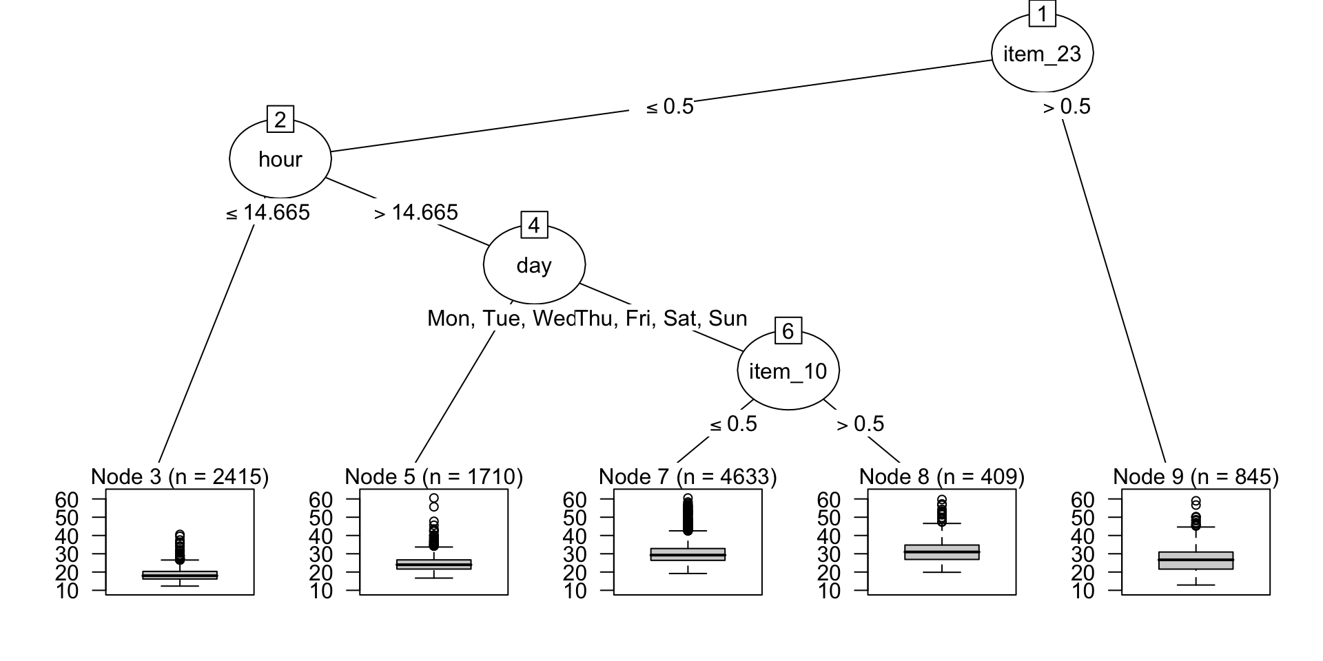
rgr_fit |>
  as.party(tree = 100, data = modeldata::deliveries) |>
  plot()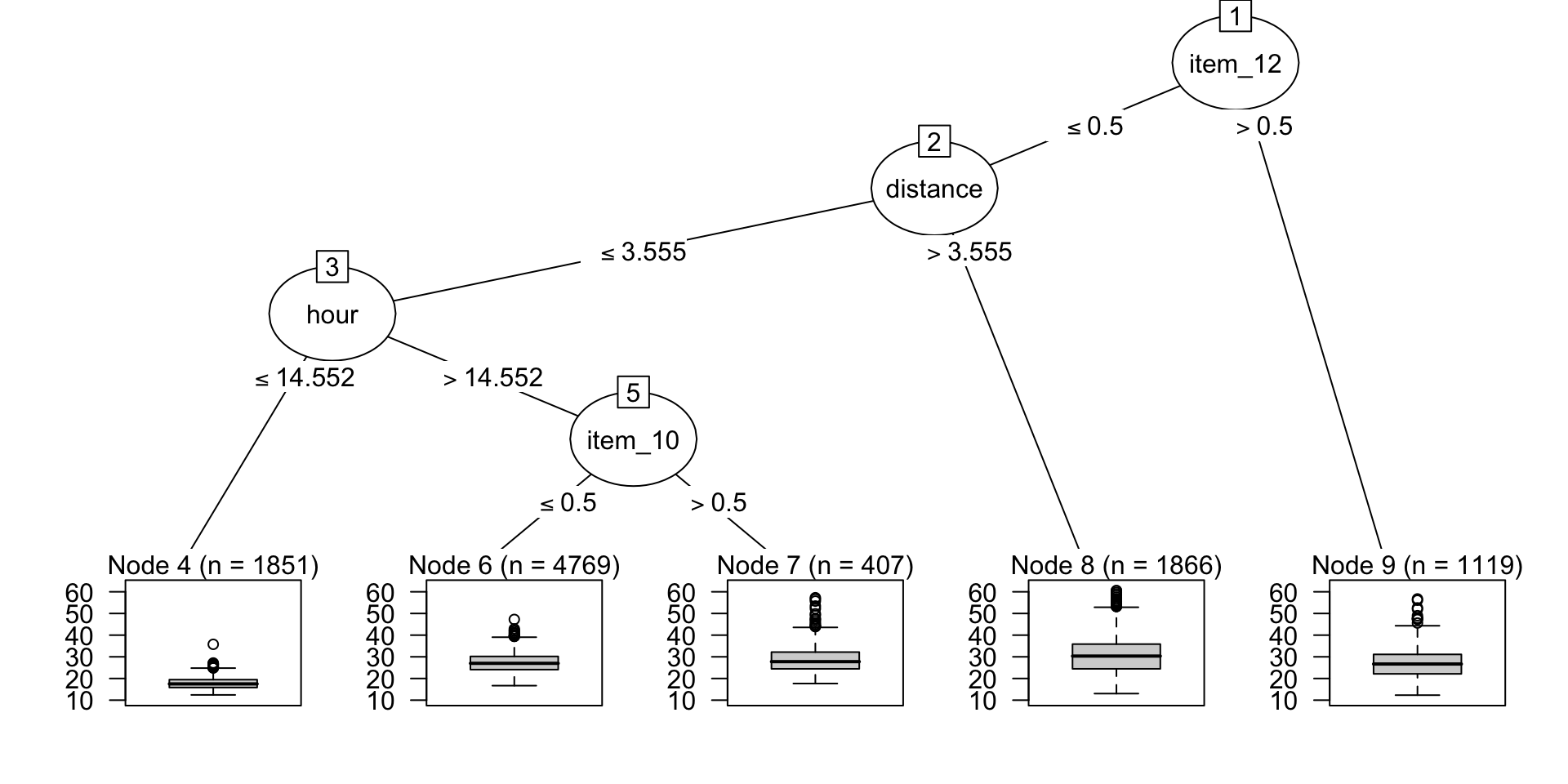
rgr_fit |>
  as.party(tree = 1000, data = modeldata::deliveries) |>
  plot()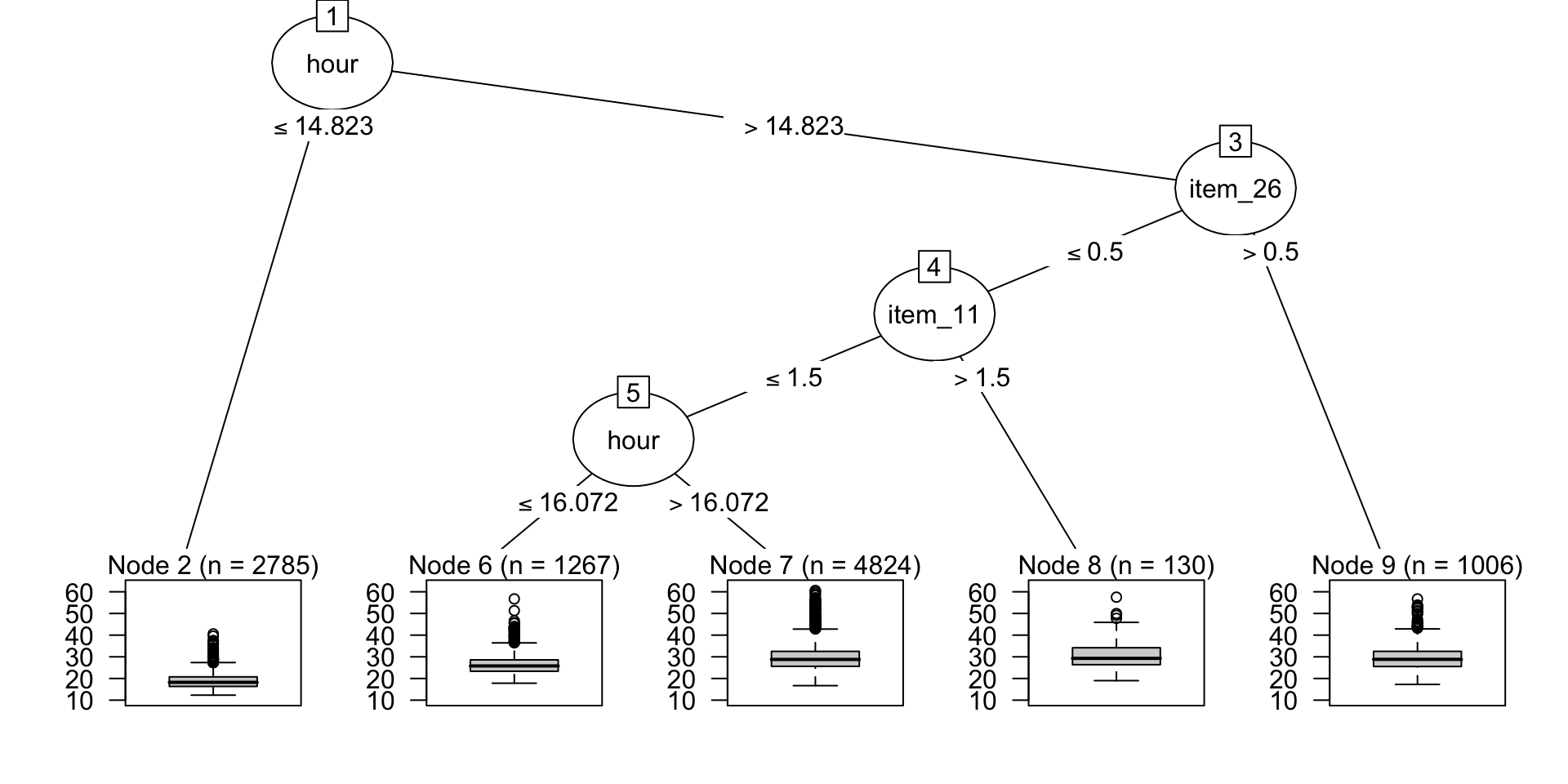
Which Predictors Were Used?#
Since trees automatically conduct feature selection as the model is trained, it helps to know which ones are actually used by the model. The active_predictors() function does just that:
rgr_vars <- active_predictors(rgr_fit, tree = 1:1000)
rgr_vars
# A tibble: 1,000 × 2
active_predictors tree
<list> <int>
1 <chr [4]> 1
2 <chr [5]> 2
3 <chr [3]> 3
4 <chr [4]> 4
5 <chr [4]> 5
6 <chr [3]> 6
7 <chr [3]> 7
8 <chr [7]> 8
9 <chr [3]> 9
10 <chr [6]> 10
# ℹ 990 more rows
# The column names are in a nested vector:
rgr_vars$active_predictors[[1]]
[1] "day" "hour" "item_10" "item_23"
# We can expand the list too:
rgr_vars |>
  unnest(cols = c(active_predictors))
# A tibble: 4,306 × 2
active_predictors tree
<chr> <int>
1 day 1
2 hour 1
3 item_10 1
4 item_23 1
5 day 2
6 distance 2
7 item_10 2
8 item_12 2
9 item_26 2
10 hour 3
# ℹ 4,296 more rows
How often are predictors used?
rgr_vars |>
  unnest(cols = c(active_predictors)) |>
  count(active_predictors) |>
  arrange(active_predictors)
# A tibble: 30 × 2
active_predictors n
<chr> <int>
1 day 516
2 distance 507
3 hour 623
4 item_01 329
5 item_02 131
6 item_03 57
7 item_04 66
8 item_05 26
9 item_06 92
10 item_07 91
# ℹ 20 more rows
How many predictors are used in each rule (on average)? A rule is the full logical statement that defines the path to the terminal nodes.
rgr_vars |>
  mutate(num_vars = map_int(active_predictors, ~ length(.x))) |>
  summarize(mean_num_vars = mean(num_vars))
# A tibble: 1 × 1
mean_num_vars
<dbl>
1 4.31
Many packages can compute variable importance scores for each predictor but each has a different interface. The lorax package has an accessor function to pull these from the model called var_imp():
var_imp(rgr_fit)# A tibble: 30 × 2
term estimate
<chr> <dbl>
1 hour 108892.
2 day 16054.
3 distance 25689.
4 item_01 673.
5 item_02 86.3
6 item_03 30.4
7 item_04 43.7
8 item_05 11.0
9 item_06 50.1
10 item_07 55.2
# ℹ 20 more rows
Examining Rules#
We can also get detailed information on the model’s rules (for each tree). Using the same ranger model fit:
rgr_rules <- extract_rules(rgr_fit, data = modeldata::deliveries)
rgr_rules
# A tibble: 5 × 3
id rules tree
<int> <list> <int>
1 3 <language> 1
2 5 <language> 1
3 7 <language> 1
4 8 <language> 1
5 9 <language> 1
# With components
rgr_rules$rules[[1]] |> class()
[1] "call"
rgr_rules$rules[[1]]item_23 <= 0.5 & hour <= 14.6645
We can compute on these and/or use them to determine which specific data were contained in the terminal node:
modeldata::deliveries |> filter(!!rgr_rules$rules[[1]])# A tibble: 2,415 × 31
time_to_delivery hour day distance item_01 item_02 item_03 item_04 item_05
<dbl> <dbl> <fct> <dbl> <int> <int> <int> <int> <int>
1 16.1 11.9 Thu 3.15 0 0 2 0 0
2 19.6 13.0 Sat 3.35 1 0 0 1 0
3 17.4 11.9 Sun 2.75 0 2 1 0 0
4 18.0 12.1 Tue 2.4 0 0 0 1 0
5 22.1 14.4 Thu 2.69 0 0 0 0 0
6 17.6 12.9 Sat 2.47 0 1 0 0 0
7 17.0 12.3 Sat 3.88 0 0 0 0 0
8 19.5 13.5 Tue 3.55 0 0 0 0 0
9 17.6 12.9 Fri 2.88 0 0 1 1 0
10 21.6 14.3 Sat 3 0 0 0 1 0
# ℹ 2,405 more rows
# ℹ 22 more variables: item_06 <int>, item_07 <int>, item_08 <int>,
# item_09 <int>, item_10 <int>, item_11 <int>, item_12 <int>, item_13 <int>,
# item_14 <int>, item_15 <int>, item_16 <int>, item_17 <int>, item_18 <int>,
# item_19 <int>, item_20 <int>, item_21 <int>, item_22 <int>, item_23 <int>,
# item_24 <int>, item_25 <int>, item_26 <int>, item_27 <int>
A List of Methods#
Here are the details of which models and methods are supported in the first CRAN version:
| class | var_imp | active_predictors | as.party | extract_rules |
|---|---|---|---|---|
| bart | n/a | ✔ | ✔ | ✔ |
| C5.0 | n/a | ✔ | ✔ | ✔ |
| cforest | ✔ | ✔ | n/a | ✔ |
| cubist | ✖ | ✔ | ✖ | ✔ |
| grf | ✔ | ✔ | ✔ | ✔ |
| lgb.Booster | ✔ | ✔ | ✔ | ✔ |
| ObliqueForest | ✔ | ✔ | ✖ | ✔ |
| party | ✔ | ✔ | n/a | ✔ |
| randomForest | ✔ | ✔ | ✔ | ✔ |
| ranger | ✔ | ✔ | ✔ | ✔ |
| rpart | ✔ | ✔ | n/a | ✔ |
| xgb.Booster | ✔ | ✔ | ✔ | ✔ |
Note that as.party.rpart() is in the partykit package and that cforest is made out of party objects.
What’s Next?#
We’ll work on adding CatBoost models to the list of supported methods. Please add an issue if there are other aspects of trees that should be quantified in these models.